Word Cloud Viz

Let’s find some customer comments to parse:

For this example I’m going to point to a BestBuy page for HP’s InstantInk product. The code below will read in their page and grab just the comments and add that to a data frame. It then repeats that process for the next 329 pages worth of comments. The code captures about 6600 customer comments. Imagine reading through all 6600 comments manually looking for themes?

Note…this type of scraping is generally frowned upon by the sites who own the data. That’s why I commentted the scraping parts out after running once and saving the raw data as a csv. It’s probably not a huge deal to just scrape once, but if you build something like this into your daily Product Management workflow you’ll probably end up getting your ip address blocked by the site owner. Be nice and be careful scraping sites.

# Environment
library(rvest)

## Loading required package: xml2

library(tidyverse)

## ── Attaching packages ────────────────────────────────────────────────────────────────────────────────────────────────────────── tidyverse 1.3.0 ──

## ✓ ggplot2 3.3.0     ✓ purrr   0.3.3
## ✓ tibble  2.1.3     ✓ dplyr   0.8.5
## ✓ tidyr   1.0.2     ✓ stringr 1.4.0
## ✓ readr   1.3.1     ✓ forcats 0.5.0

## ── Conflicts ───────────────────────────────────────────────────────────────────────────────────────────────────────────── tidyverse_conflicts() ──
## x dplyr::filter()         masks stats::filter()
## x readr::guess_encoding() masks rvest::guess_encoding()
## x dplyr::lag()            masks stats::lag()
## x purrr::pluck()          masks rvest::pluck()

library(stringr)
library(tidytext)
library(tm)

## Loading required package: NLP

## 
## Attaching package: 'NLP'

## The following object is masked from 'package:ggplot2':
## 
##     annotate

library(wordcloud2)

# Target URL to scrape
#base_url <- "https://www.bestbuy.com/site/reviews/hp-instant-ink-50-page-monthly-plan-for-select-hp-printers/5119176"

# Load page
#page <- read_html(base_url)

# Scrape just the comments from the page
#comments <- page %>%
#     html_nodes(".pre-white-space") %>%
#     html_text() %>%
#     tbl_df()

# Be nice if you're using this approach...don't over tax someone's website.
# Loop to do the same over pages 2 to 330
#for (i in 2:330) {
#     url <- paste0(base_url, "?page=", i)
#     page <- read_html(url)
     
#     new_comments <- page %>%
#          html_nodes(".pre-white-space") %>%
#          html_text() %>%
#          tbl_df()
     
#     comments <- rbind(comments,new_comments)
#}


#write_csv(comments, "../../data/ink_comments.csv")

comments <- read_csv("../../data/ink_comments.csv")

## Parsed with column specification:
## cols(
##   value = col_character()
## )

Unpack all of those comments

To make use of all of those comments, the first step is to break the comments into a long list of individual words.

Next, using the TidyText package we can obtain a list of ‘stop words’ and filter those out from our long list. Stop words are words that just common words like ‘the’ ‘and’ ‘but’ and such that don’t really help in our analysis.

Once we’ve filtered out the stop words we can count the instances of each word.

# Unnest each word from the long list of comments
text <- unnest_tokens(comments, word, value)


# Summarize words rejecting stopwords
word_count <- text %>%
     anti_join(get_stopwords(), by = "word") %>%
     count(word, sort = TRUE) 

Determining the Sentiments for each word

The TidyText package also contains datasets which include sentiment information for a huge number of words. For example, “convenient” is tagged as a positive word, whereas “hassle” is considered negative.

# Join sentiments
word_count <- word_count %>%
     inner_join(get_sentiments("bing"), by = "word")

Render some word clouds

I like the wordcloud2 package for rendering this illustrations. Wordcloud2 needs a data frame with a column for word and another column for the frequency for each word. You can play around with fonts and such. Here, I just picked colors for Positive versus Negative word clouds

# Positive and negative wordclouds
pos_words <- word_count %>%
     filter(sentiment == "positive")

wordcloud2(pos_words, color = 'random-light')

neg_words <- word_count %>%
     filter(sentiment == "negative")

wordcloud2(neg_words, color = 'random-dark')

Anything else?

While word clouds effectively communicate the relative importance of words, sometimes it’s helpful to look at the data as seen below.

# Positive and negative frequency bar plots
pos_words %>%
     arrange(-n) %>%
     head(n =20) %>%
     ggplot(aes(x= reorder(word, n), y = n)) +
     geom_bar(stat = 'identity', fill = 'blue', alpha = .6) +
     coord_flip() +
     theme_minimal() +
     labs(title = "Frequency of top 20 Positive words", x = "")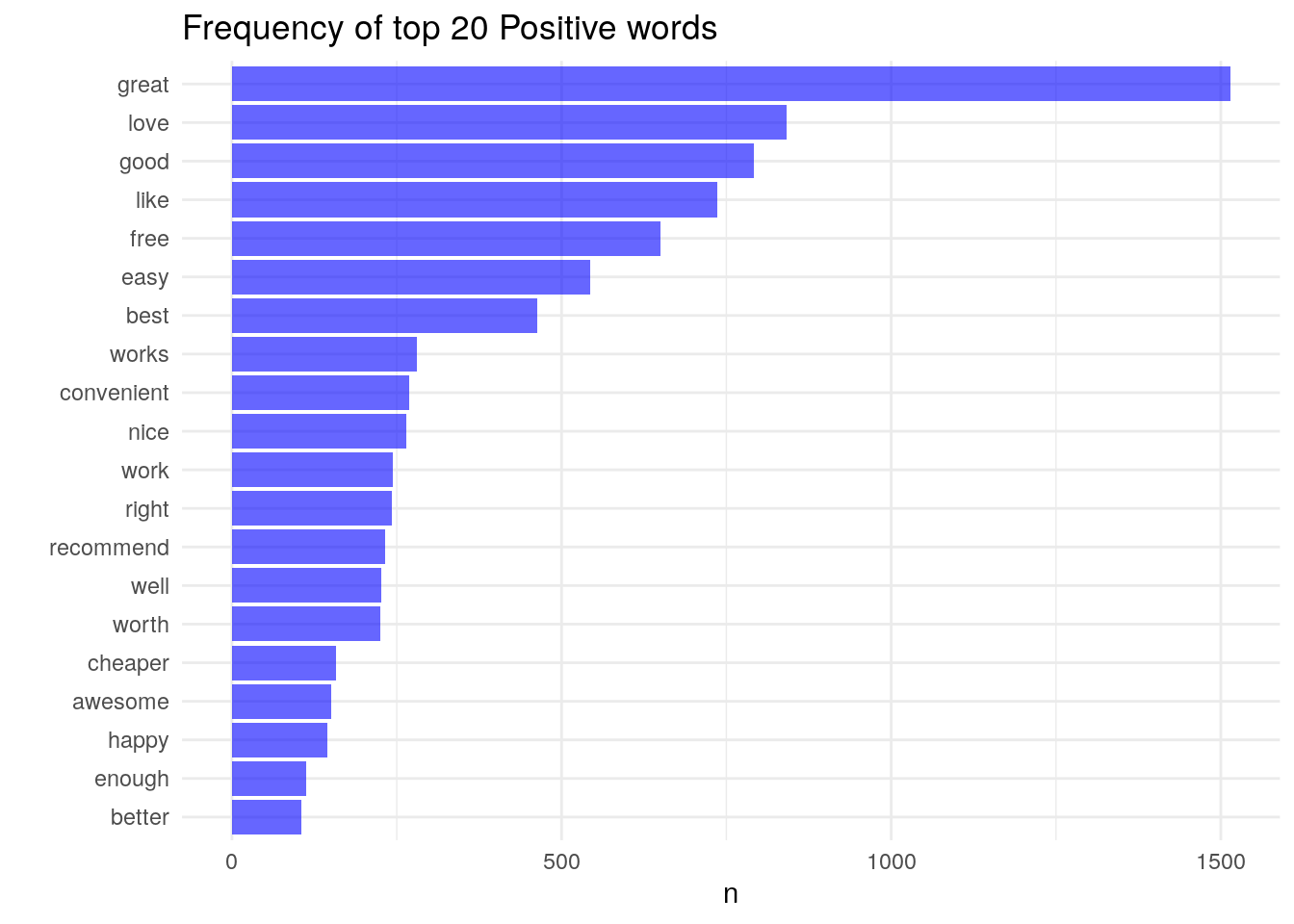

neg_words %>%
     arrange(-n) %>%
     head(n =20) %>%
     ggplot(aes(x= reorder(word, n), y = n)) +
     geom_bar(stat = 'identity', fill = 'red', alpha = .6) +
     coord_flip() +
     theme_minimal() +
     labs(title = "Frequency of top 20 Negative words", x = "")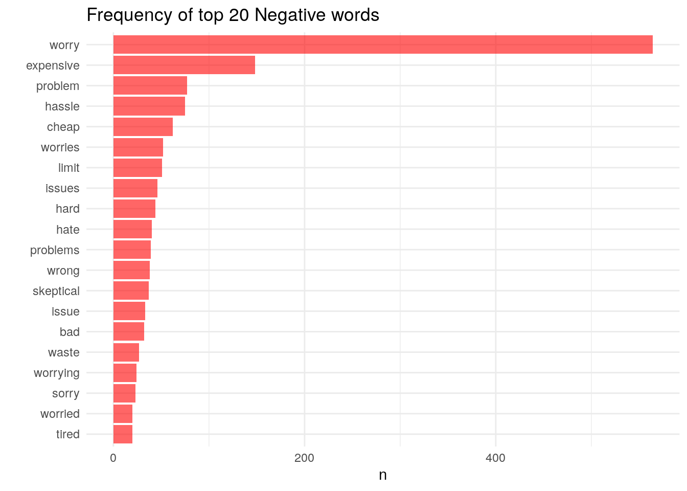

# quick summary of number of words
sum(pos_words$n)

## [1] 11540

sum(neg_words$n)

## [1] 2458

# ratio of good to bad
sum(pos_words$n)/sum(neg_words$n)

## [1] 4.694874

Finally

These tools can be helpful, but you still need to do your manual work here. The negative word cloud above illustrated that many comments included the word “worry”. However, reading through a few comments we see things like “It’s great not to worry about…” and “I never have to worry about running to the store”

Clearly in this context the word “worry” is actually a positive thing. This doesn’t discount the approach, it just illustrates that as the analyst you need to use every tool in your kit to best understand what’s going on.